(1) Extract keyframes
Run: VideoSummarization.exe or run from Visual studio, pass Video Path as parametter
(2) Extract features:
- Color moments and LBP features:
Run script: extract_feature_leduy.sh from command, view http://nii-kaori.blogspot.com/2010/07/trecvid-datasets-global-feature.html to get detail description
- Optical flow - motion histogram
Run matlab command:
ComputeOpticalFlow(ftFilePath, frameLstFilePath, frameLstRoot, runFromPos, runToPos, gridX, gridY, piStep)
+ ftFilePath: Đường dẫn đến file feature muốn tạo
+ frameLstFilePath: File chứa danh sách các frame muốn extract feature
+ frameLstRoot: Đường dẫn đến thư mục chứa các frames
+ runFromPos: Bắt đầu chạy từ frame nào (mục đích là để chạy song song nhiều thread)
+ rungToPos: Chạy đến frame nào
+ gridX: chia lưới ảnh theo chiều ngang thành bao nhiêu
+ gridY: chia lưới ảnh theo chiều dọc thành bao nhiêu
+ piStep: bước chia để quantize optical flow tạo histogram (ví dụ piStep = 4 --> khoảng chia độ: [-pi:pi/4:pi] tức là quantize thành 8 hướng chính
(3) Feature Fusion
Trước khi fusion các features cần thực hiện việc chuẩn hóa các features để khi kết hợp vai trò của các feature như nhau
3.1. Scale các feature về đoạn [0 1]: giá trị của mỗi bin chỉ rơi vào trong khoảng [0,1]
Run matlab command:
ScalingFeature(ftFilePath)
+ ftFilePath: Đường dẫn đến file chứa feature cần scale
3.2. Normalize các feature về đoạn [0 1]: giá trị mỗi bin nằm trong khoảng [0 1] và tổng giá trị của các bin trong 1 vector = 1
Run matlab command:
NormalizeFeature(ftFilePath)
+ ftFilePath: Đường dẫn đến file chứa feature cần normalize
3.3. Bin-based normalize: (Normalize by standard deviation) Đây là bước bắt buộc phải làm nếu training bằng SVM
Run matlab command:
NormalizeFeatureByDeviation(ftFilePath)
+ ftFilePath: Đường dẫn đến file chứa feature cần normalize
Tiếp theo là concatenate các feature lại theo thứ thự: colormoment + lbp + motion
Run php script:
FeatureConcatenate(ftDesFilePath, ftScrFilePath1, ftScrFilePath2, ftScrFilePath3)
+ ftDesFilePath: Đường dẫn đến file feature muốn tạo
+ ftSrcFilePath1: Đường dẫn đến file feature color moments
+ ftSrcFiletPath2: Đường dẫn đến file feature LBP
+ ftSrcFilePath3: Đường dẫn đến file feature motion
(4) Kmean - Clustering
Run matlab command:
SaveClusteringLabel2File(clusteringFilePath, ftFilePath, numberOfCluster)
+ clusteringFilePath: Đường dẫn đến file chứa label (output)
+ ftFilePath: Đường dẫn đến file feature
+ numberOfCluster: Số lượng cluster
(5) Build scoring matrix
Run matlab command:
BuildScoringMatrixOfClusterSequence(clusterFilePath)
+ clusterFilePath: Đường dẫn đến file chứa cluster label
(6) Find all sub-sequence repeated in the video
Rung matlab command
SaveSequenceAlignment2RankListFile(scoringMatrixFilePath)
+ scoringMatrixFilePath: Đường dẫn đến file chứa scoring
(7) Clustering takes of the same scene
Run php script (dùng web browser để chạy)
http://localhost/videosummarization/TakesClustering.php
+ Chọn số lượng cluster tương ứng, sẽ cho ra các kết quả nhóm take khác nhau
(8) Evaluate
- Evaluate theo tiêu chí tự propose (so độ overlap giữa take của system và take của ground truth)
Run php script (dùng web browser để chạy)
http://localhost/videosummarization/SceneTakeEvaluation.php
- Evaluate bằng cách: So sánh giữa 2 cách clustering (ground truth clustering, system clustering) khi đó coi mỗi scene là một cluster của các frame và mỗi take là một cluster của các frame
Run matlab command:
SceneTakeEvaluateByRI(gtClusteringFilePath, systemClusteringFilePath)
+ gtClusteringFilePath: Đường dẫn đến file scene take ground truth
+ systemClusteringFilePath: Đường dẫn đến file scene take của hệ thống
Thứ Năm, 16 tháng 12, 2010
Thứ Năm, 18 tháng 11, 2010
Video summarization (5)
1. Extract feature (cm & lbp)
2. Clustering
3. Build Scoring matrix
4. Build Alignment subsequence
(continue...)
2. Clustering
3. Build Scoring matrix
4. Build Alignment subsequence
(continue...)
Thứ Tư, 17 tháng 11, 2010
Video Summarization (4)
Werner - Bailer 's frame work
1) Loại junk frames
2) Chạy SBD (Shot Boundary Detection) để chia video thành các parts, in general (assumption của tác giả) là các part sẽ chứa 1 hoặc nhiều takes - trong trường hợp lý tưởng là mỗi part chứa 1 take
3) Dùng pair-wise similarity để tính ra các đoạn con giống nhau trong các part --> lưu là take candidates (vì thông thường mỗi take được quay nhiều lần --> do đó trong các parts khác nhau sẽ có các đoạn giống nhau)
4) Chạy linkage-hierarchical clustering các take candidates
5) Sampling để lấy ra các frame đại diện dùng làm summary clip
Để tính similarity giữa 2 parts p1 vaf p2
(1) Extract feature cho part1 và part2
(2) Vì trong 1 part có nhiều frame nên sampling các frames --> sau đó extract feature cho các frame này (sử dụng khá nhiều các feature khác nhau biểu diễn cho một keyframe: color moment, edge orientation)
- Feature của 1 part = concatenate Feature của các keyframes (sampling từ part)
- Feature của 1 keyframe = concatenate các features khác nhau
Similarity giữa 2 parts: S(p1, p2) = 1 - Normalize{LCSS(p1, p2)} (còn phần chuẩn hóa loằng ngoằng nữa, nhưng bản chất là như vậy)
Tại sao LCSS: vì mỗi part có thể coi là một chuỗi các keyframe --> dùng LCSS để alignment 2 chuỗi với nhau tìm ra các đoạn giống nhau
Độ đo similarity giữa 2 keyframe đơn giản là L2 (Khoảng cách Euclide giữa 2 feature tương ứng với 2 keyframes)
Video Summarization (3)
Emili Dumont's frame work
Đầu tiên là loại bỏ các junk frame (color bars, clap-boards, mono-color-frames...). Sau đó
1) Từ video ban đầu chia thành các segment 1 second
Lý do: 1 second nhỏ nhất để có thể nhận ra một cảnh + take overlap nếu có thì cũng không ảnh hưởng
2) Extract feature cho các 1-second-segments --> Lấy trung bình trên 25 frames (dùng HSV histogram)
3) Hierarchical clustering: Sau bước này, tại mỗi level của clustering: video sẽ được biểu diễn như một chuỗi string, mỗi ký tự là label của cluster của frame tương ứng
4) Sử dụng thuật toán smith-waterman để tìm ra các chuỗi con lặp lại trong nó --> lưu dưới dạng rank list chuỗi đầu tiên là chuỗi tốt nhất
5) Scene boudary detection: để tìm scene boudary --> build alignment matrix --> tính rect(f)
6) Take selection and re-take removal: Chọn chuỗi dài nhất các frame liên tiếp mà không có frame nào aligned với nhau là take
7) Summary clip generation: đến bước này toàn bộ các frame un-interesting đã bị loại bỏ, tuy nhiên duration vẫn vượt quá time uper-limited --> phải tiến hành chọn các frames đại diện trong mỗi take để build summary clip
Thứ Năm, 21 tháng 10, 2010
Thứ Hai, 18 tháng 10, 2010
Video summarization (2)
Tên bài báo: Unsupervised Summarization of Rushes Videos - Yang Liu Hong Kong polytechnic University
Input: BBC Rushes Video
Step 1. Video Segmentation
Step 2. Shot clustering
Step 3. Redundant Information and Junk Clip removal
Step 4. Final Summary Generation
Output: Video summary
Ở đây 2 bước 1 và 2 được gộp vào xử lý chung, sử dụng qui hoạch động để gán segment nào thuộc vào cluster nào
Bước số 3: Loại bỏ các redundant và junk bằng cách
Loại bỏ redundant: Mỗi cluster chỉ lấy ra clips dài nhất
Để loại junk clips: tính mean values of gradient theo vertical direction, so sánh với threshold để chỉ ra clips đó là normal hay junk
Bước 4:
- Tính toán số keyframe tối đa được lấy (dựa vào tiêu chí total of length in each summary < 4% original video)
- Keyframes extract:
+ Cách 1: sử dụng lấy mẫu đều: uniform sampling
+ Cách 2: k mean cluster
- Extend each keyframe to one-second clips and concatenating them orderly to get final summary
Video summarization (1)
Tên bài báo: Rushes Video Summarization by Object and Event Understanding - TRECVID 2007 workshop
Feng Wang - City Uninversity of Hong Kong 's method
Để có được summary video từ rushes video, đại học Hong Kong làm như sau
(rushes video ở đây là BBC rushes - Các đoạn phim, trong đó có thể chứa rất nhiều thông tin dư thừa bên trong)
1. Từ video chạy thuật toán shot detection: theo bài "Video partitioning through Temporal slide analysis" - C.W.Ngo
Sử dụng thuật toán extract keyframe theo bài: "An Innovative Algorithm for Keyframe Extraction in Video summarization" - Journal of realtime Image processing 2006
2. Junk Shot Filtering: Loại bỏ các shot sau
- Quá ngắn: < 10 frame/shot
- Các shot chỉ chứa: color bar (dải màu hay nhìn thấy trên TV khi chưa phát gì), các gray, black frame: phương pháp so sánh histogram của các keyframes với các example color bar hay các gray, black frame có sẵn
3. Subshot partition: Chia các shot thành các subshot, đây là bước khá then chốt và Feng Wang sử dụng khác nhiều trick ở đây
3.1. Tại sao phải chia nhỏ các shot thành các subshots?
Trong rushes video thì các shots không chỉ chứa nội dung phim mà còn các cảnh dư thừa: ví dụ trao đổi giữa đạo diễn và diễn viên, cảnh được đóng đi đóng lại nhiều lần nhắm đảm bảo độ chất lượng...
3.2. Phương pháp partition
Vấn đề ở đây là cần tìm ra các điểm bắt đầu và kết thúc của một subshot
a) Sử dụng thuật toán based on camera motion estimation, sau đó sử dụng Hierarchical Hidden Markov Model cho việc phân loại: stock, outtake, shaky và partition một shot thành các subshot theo 3 loại này
b) Tìm các retake scence: thông thường khi bắt đầu một cảnh quay, đạo diễn thường giơ tấm bảng (trên đó ghi cảnh bao nhiêu...) --> dựa vào điều này có thể lấy các frame có chứa tấm bảng này làm điểm bắt đầu của một subshot mới
c) Dựa vào các khẩu lệnh của đạo diễn để xác định điểm bắt đầu và điểm kết thúc của một subshot. Ví dụ "action", "cut"
d) feature cuối cùng là audio
4. Repetitive Subshot Removal
Đến đây chúng ta đã có các subshot, trong đó chỉ chứa nội dung liên quan đến phim. Tuy nhiên vẫn có các đoạn dư thừa: thông thường một đoạn kịch bản thường được đóng đi đóng lại nhiều lần --> nhiều subshots giống nhau --> cần được loại bỏ
Với 2 subshot: s1, s2 có hai trường hợp cần quan tâm
- s1 là subshot của s2 --> đơn giản là loại bỏ s1
- s1 và s2 là lặp lại của nhau: trường hợp này chỉ chọn subshot cuối và không loại bỏ tất cả subshot còn lại
5. Video Summarization
Đến đây đã loại bỏ các junk shot, các repetive subshot. Các subshot còn lại hầu hết là liên quan trực tiếp đến phim và useful cho việc summary
5.1. Extract feature from video
5 loại feature được extract
- Set of object
- Set of object motion activity
- List of camera motion
- The scene changes giữa các neighboring frames
- Dialogue or speech clips
5.2. Summarization
Chia các subset thành các clips, mỗi clips có độ dài 1 giây (tức là khoảng 25 frame) và overlap với clips trước 300ms
Mục đích là đi chọn tập V = {v1, v2, ...vd} that are most representive
Step1. Initialize Sum = {};
C: tập các video clips sắp xếp theo độ representability
Step2: Chọn một cj thuộc C với representability cao nhất
Sum = Sum + cj
Step3: Loại bỏ tất cả các clips cp mà Rep(cj, cp) > threshold
Step4: Go to step2 nếu C chưa rỗng
Chủ Nhật, 10 tháng 10, 2010
Thứ Ba, 5 tháng 10, 2010
Thứ Năm, 30 tháng 9, 2010
Laplace operator
http://en.wikipedia.org/wiki/Laplace_operator
Laplace operator được định nghĩa như sau:
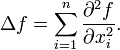
The Laplace operator is a second order differential operator in the n-dimensional Euclidean space, defined as the divergence (∇·) of the gradient (∇ƒ). Thus if ƒ is a twice-differentiable real-valued function, then the Laplacian of ƒ is defined by
Lại có công thức của devergence như sau:
The divergence of a vector field can be defined in any number of dimensions. If
 and
and  , define
 (2)
(2)
Chủ yếu chúng ta quan tâm đến công thức của toán tử laplace cho 2 chiều
In polar coordinates,
Laplace operator được định nghĩa như sau:
The Laplace operator is a second order differential operator in the n-dimensional Euclidean space, defined as the divergence (∇·) of the gradient (∇ƒ). Thus if ƒ is a twice-differentiable real-valued function, then the Laplacian of ƒ is defined by
 (1)
(1)
Lại có công thức của devergence như sau:
The divergence of a vector field can be defined in any number of dimensions. If
 and , define
 (2)
(2)Chủ yếu chúng ta quan tâm đến công thức của toán tử laplace cho 2 chiều
Two dimensions
The Laplace operator in two dimensions is given by
In polar coordinates,

Divergence
http://en.wikipedia.org/wiki/Divergence
In vector calculus, divergence is an operator that measures the magnitude of a vector field's source or sink at a given point, in terms of a signed scalar. More technically, the divergence represents the volume density of the outward flux of a vector field from an infinitesimal volume around a given point. For example, consider air as it is heated or cooled. The relevant vector field for this example is the velocity of the moving air at a point. If air is heated in a region it will expand in all directions such that the velocity field points outward from that region. Therefore the divergence of the velocity field in that region would have a positive value, as the region is a source. If the air cools and contracts, the divergence is negative and the region is called a sink.
Định nghĩa của divergence rất khó hiểu như sau:
More rigorously, the divergence of a vector field F at a point p is defined as the limit of the net flow of F across the smooth boundary of a three dimensional region V divided by the volume of V as V shrinks to p. Formally,
Let x, y, z be a system of Cartesian coordinates on a 3-dimensional Euclidean space, and let i, j, k be the corresponding basis of unit vectors.
The divergence of a continuously differentiable vector field F = U i + V j + W k is equal to the scalar-valued function:
In vector calculus, divergence is an operator that measures the magnitude of a vector field's source or sink at a given point, in terms of a signed scalar. More technically, the divergence represents the volume density of the outward flux of a vector field from an infinitesimal volume around a given point. For example, consider air as it is heated or cooled. The relevant vector field for this example is the velocity of the moving air at a point. If air is heated in a region it will expand in all directions such that the velocity field points outward from that region. Therefore the divergence of the velocity field in that region would have a positive value, as the region is a source. If the air cools and contracts, the divergence is negative and the region is called a sink.
Định nghĩa của divergence rất khó hiểu như sau:
More rigorously, the divergence of a vector field F at a point p is defined as the limit of the net flow of F across the smooth boundary of a three dimensional region V divided by the volume of V as V shrinks to p. Formally,

Let x, y, z be a system of Cartesian coordinates on a 3-dimensional Euclidean space, and let i, j, k be the corresponding basis of unit vectors.
The divergence of a continuously differentiable vector field F = U i + V j + W k is equal to the scalar-valued function:

Gradient
http://en.wikipedia.org/wiki/Gradient
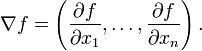
In vector calculus, the gradient of a scalar field is a vector field which points in the direction of the greatest rate of increase of the scalar field, and whose magnitude is the greatest rate of change.
Gradient là một vector
Ví dụ: Nhiệt độ trong một căn phòng là một đại lượng vô hướng T. Giả sử T không thay đổi theo thời gian, tại mỗi điểm trong căn phòng tọa độ (x, y, z) có một nhiệt độ nhất định, T(x, y, z)
Việc tính gradient của T tại một điểm, hướng của vector gradient sẽ chỉ cho ta biết hướng nào nhiệt độ tăng nhanh nhất tại điểm đó và độ lớn của vector gradient sẽ cho biết nhiệt độ tăng nhanh như thế nào
Definition:

 The gradient of the function f(x,y) = −(cos2x + cos2y)2 depicted as a vector field on the bottom plane
The gradient (or gradient vector field) of a scalar function is denoted
  or
or  where
where  (the nabla symbol) denotes the vector differential operator, del. The notation
  is also used for the gradient. The gradient of f is defined to be the vector field whose components are the partial derivatives of f. That is:
The gradient of a vector is
is 
or the transpose of the Jacobian matrix .
.
It is a second-rank tensor.
More generally, the gradient may be defined using the exterior derivative:
In vector calculus, the gradient of a scalar field is a vector field which points in the direction of the greatest rate of increase of the scalar field, and whose magnitude is the greatest rate of change.
Gradient là một vector
Ví dụ: Nhiệt độ trong một căn phòng là một đại lượng vô hướng T. Giả sử T không thay đổi theo thời gian, tại mỗi điểm trong căn phòng tọa độ (x, y, z) có một nhiệt độ nhất định, T(x, y, z)
Việc tính gradient của T tại một điểm, hướng của vector gradient sẽ chỉ cho ta biết hướng nào nhiệt độ tăng nhanh nhất tại điểm đó và độ lớn của vector gradient sẽ cho biết nhiệt độ tăng nhanh như thế nào
Definition:

The gradient (or gradient vector field) of a scalar function
is denoted or where (the nabla symbol) denotes the vector differential operator, del. The notation is also used for the gradient. The gradient of f is defined to be the vector field whose components are the partial derivatives of f. That is:The gradient of a vector
is or the transpose of the Jacobian matrix
.It is a second-rank tensor.
More generally, the gradient may be defined using the exterior derivative:

Thứ Tư, 29 tháng 9, 2010
LBP - Local binary patterns
http://www.scholarpedia.org/article/Local_Binary_Pattern
LBP là descriptor cho texture extraction
Lý thuyết về LBP khá dễ hiểu, được đưa ra đầu tiên vào năm 1996 bởi Ojala
Fig. 2 for an example of LBP computation.

Ý tưởng của LBP là tại mỗi sample point (center point), so sánh sự khác nhau giữa center point này và P điểm lân cận trên bán kính R (thường là 8 điểm lân cận, bán kính 1 tức là các điểm liền kề ngay center point)
Sau đó mã hóa hình trên, như vậy nếu mã hóa (8,1) neighborhood sẽ có 2^8 = 256 partern, tuy nhiên LBP không dùng 256 partern này làm các label mà định nghĩa thêm khái niệm uniform patterns mục đích là giảm chiều dài của feature vector
A local binary pattern is called uniform if the binary pattern contains at most two bitwise transitions from 0 to 1 or vice versa when the bit pattern is traversed circularly
For example: the patterns 00000000 (0 transitions), 01110000 (2 transitions) and 11001111 (2 transitions) are uniform whereas the patterns 11001001 (4 transitions) and 01010010 (6 transitions) are not
Sau đó mỗi uniform pattern sẽ được gán một nhãn (label), tất cả các pattern còn lại gán chung một label
Như vậy nếu dùng (8,1) neighborhood thì sẽ có 256 pattern, trong đó có 58 uniform, nên suy ra số chiều của một bin trong LBP là 59
SpatialTemporal LBP (LBP kết hợp không gian và thời gian)
Như đã trình bày ở trên thì LBP chỉ liên quan đến không gian, chưa có mỗi liên hệ với thời gian. Zhao and Pietikäinen 2007 đưa ra khái niệm VLBP, thực chất là mở rộng của LBP thêm chiều thời gian
The neighborhood of each pixel is thus defined in three dimensional space. Then, similarly to LBP in spatial domain, volume textons can be defined and extracted into histograms. Therefore, VLBP combines motion and appearance together to describe dynamic textures.
To make VLBP computationally simple and easy to extend, an operator based on co-occurrences of local binary patterns on three orthogonal planes (LBP-TOP) was also introduced. LBP-TOP considers three orthogonal planes: XY, XT and YT, and concatenates local binary pattern co-occurrence statistics in these three directions as shown in Fig.1. The circular neighborhoods are generalized to elliptical sampling to fit to the space-time statistics.

Một đặc điểm nữa là LBP kết hợp với HOG rất tốt trong bài toán classify human (human vs non human)
Convolution
Đây là định nghĩa:
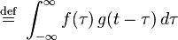
The convolution of ƒ and g is written ƒ∗g, using an asterisk or star. It is defined as the integral of the product of the two functions after one is reversed and shifted. As such, it is a particular kind of integral transform:
While the symbol t is used above, it need not represent the time domain. But in that context, the convolution formula can be described as a weighted average of the function ƒ(τ) at the moment t where the weighting is given by g(−τ) simply shifted by amount t. As t changes, the weighting function emphasizes different parts of the input function.
More generally, if f and g are complex-valued functions on Rd, then their convolution may be defined as the integral:
Một số tính chất của convolution
 .
.
No algebra of functions possesses an identity for the convolution. The lack of identity is typically not a major inconvenience, since most collections of functions on which the convolution is performed can be convolved with a delta distribution or, at the very least (as is the case of L1) admit approximations to the identity[disambiguation needed]. The linear space of compactly supported distributions does, however, admit an identity under the convolution. Specifically,
These identities hold under the precise condition that ƒ and g are absolutely integrable and at least one of them has an absolutely integrable (L1) weak derivative, as a consequence of Young's inequality. For instance, when ƒ is continuously differentiable with compact support, and g is an arbitrary locally integrable function,
In the discrete case, the difference operator D ƒ(n) = ƒ(n + 1) − ƒ(n) satisfies an analogous relationship:
The convolution of ƒ and g is written ƒ∗g, using an asterisk or star. It is defined as the integral of the product of the two functions after one is reversed and shifted. As such, it is a particular kind of integral transform:
While the symbol t is used above, it need not represent the time domain. But in that context, the convolution formula can be described as a weighted average of the function ƒ(τ) at the moment t where the weighting is given by g(−τ) simply shifted by amount t. As t changes, the weighting function emphasizes different parts of the input function.

 (
(More generally, if f and g are complex-valued functions on Rd, then their convolution may be defined as the integral:

![(f * g)[n]\ \stackrel{\mathrm{def}}{=}\
\sum_{m=-\infty}^{\infty} f[m]\, g[n - m]](http://upload.wikimedia.org/math/5/d/2/5d2777af939cdafb39a2988f1c2eae9a.png)
![= \sum_{m=-\infty}^{\infty} f[n-m]\, g[m].](http://upload.wikimedia.org/math/4/3/2/432b9d6de30ebd84ce49f993f8a3a04c.png) (
(Một số tính chất của convolution

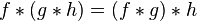

- Associativity with scalar multiplication

.No algebra of functions possesses an identity for the convolution. The lack of identity is typically not a major inconvenience, since most collections of functions on which the convolution is performed can be convolved with a delta distribution or, at the very least (as is the case of L1) admit approximations to the identity[disambiguation needed]. The linear space of compactly supported distributions does, however, admit an identity under the convolution. Specifically,

- Inverse element

- Complex conjugation

Integration
If ƒ and g are integrable functions, then the integral of their convolution on the whole space is simply obtained as the product of their integrals:
Differentiation
In the one-variable case,

These identities hold under the precise condition that ƒ and g are absolutely integrable and at least one of them has an absolutely integrable (L1) weak derivative, as a consequence of Young's inequality. For instance, when ƒ is continuously differentiable with compact support, and g is an arbitrary locally integrable function,

In the discrete case, the difference operator D ƒ(n) = ƒ(n + 1) − ƒ(n) satisfies an analogous relationship:

Chủ Nhật, 26 tháng 9, 2010
Một số khái niệm liên quan đến matrix
Phần này là bổ xung cho việc ngày xưa không được học toán bằng tiếng Anh nên nhiều thuật ngữ tiếng Anh liên quan đến matrix không biết (mặc dù được học rồi :)
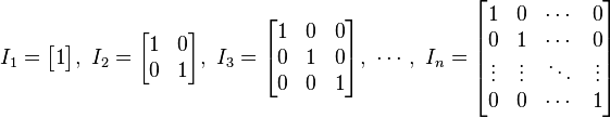
1. Identity matrix (unit matrix - ma trận đơn vị)
3. Trace (linear algebra)
In linear algebra, a Trace of an n-by-n square matrix A is defined to be sum of the elements on the main diagonal of matrix
4. Eigenvalue, Eigenvector and Eigenspace
http://en.wikipedia.org/wiki/Eigenvalue,_eigenvector_and_eigenspace
1. Identity matrix (unit matrix - ma trận đơn vị)
3. Trace (linear algebra)
In linear algebra, a Trace of an n-by-n square matrix A is defined to be sum of the elements on the main diagonal of matrix

4. Eigenvalue, Eigenvector and Eigenspace
http://en.wikipedia.org/wiki/Eigenvalue,_eigenvector_and_eigenspace
5. Eigenvalue relationships
If A is a square n-by-n matrix with real or complex entries and if λ1,...,λn are the (complex and distinct) eigenvalues of A (listed according to their algebraic multiplicities), then


Thứ Năm, 23 tháng 9, 2010
Thứ Tư, 22 tháng 9, 2010
SVM
Tìm được một blog tiếng Việt viết rất chi tiết về SVM :)
http://csstudyfun.wordpress.com/tag/support-vector-machines/page/3/
http://csstudyfun.wordpress.com/tag/support-vector-machines/page/3/
Thứ Ba, 21 tháng 9, 2010
Quy hoạch tuyến tính
http://vi.wikipedia.org/wiki/Quy_ho%E1%BA%A1ch_tuy%E1%BA%BFn_t%C3%ADnh
video for linear program (very interesting :)
http://www.youtube.com/watch?v=a2QgdDk4Xjw&feature=channel
video for linear program (very interesting :)
http://www.youtube.com/watch?v=a2QgdDk4Xjw&feature=channel
Tối ưu hóa
Tối ưu hóa:
http://vi.wikipedia.org/wiki/T%E1%BB%91i_%C6%B0u_h%C3%B3a_%28to%C3%A1n_h%E1%BB%8Dc%29
Các lĩnh vực con chính
* Quy hoạch tuyến tính (Linear programming) nghiên cứu các trường hợp khi hàm mục tiêu f là hàm tuyến tính và tập A được mô tả chỉ bằng các đẳng thức và bất đẳng thức tuyến tính (A được gọi là một khúc lồi).
* Quy hoạch số nguyên (Integer programming) nghiên cứu các quy hoạch tuyến tính trong đó một số hoặc tất cả các biến có giới hạn là các số nguyên.
* Quy hoạch bậc hai (hay quy hoạch toàn phương) (Quadratic programming) cho phép hàm mục tiêu có các toán hạng bậc hai, trong khi tập A phải mô tả được bằng các đẳng thức và bất đẳng thức tuyến tính (A được gọi là một khúc lồi).
* Quy hoạch phi tuyến (Nonlinear programming) nghiên cứu trường hợp tổng quát khi hàm mục tiêu hay các ràng buộc hoặc cả hai chứa các thành phần không tuyến tính.
* Quy hoạch ngẫu nhiên (Stochastic programming) nghiên cứu các trường hợp khi một số ràng buộc phụ thuộc vào các biến ngẫu nhiên.
* Quy hoạch động (Dynamic programming) nghiên cứu các trường hợp khi chiến lược tối ưu hóa dựa trên việc chia bài toán thành các bài toán con nhỏ hơn (nguyên lý quy hoạch động).
* Tối ưu hóa tổ hợp (Combinatorial optimization) quan tâm đến các bài toán trong đó tập các lời giải khả thi là rời rạc hoặc có thể được rút gọn về một tập rời rạc.
* Infinite-dimensional optimization nghiên cứu trường hợp khi tập các lời giải khả thi là một tập con của một không gian vô số chiều, chẳng hạn không gian các hàm số (ví dụ bài toán điều khiển tối ưu).
* Constraint satisfaction nghiên cứu trường hợp khi hàm mục tiêu f là hằng số – đây là vấn đề quan trọng của ngành Trí tuệ nhân tạo, đặc biệt là lĩnh vực Suy luận tự động (Automated reasoning).
Thứ Tư, 15 tháng 9, 2010
Linux regular expression
Metacharacter Description
. Matches any single character. For example the regular expression r.t would match the strings rat, rut, r t, but not root.
$ Matches the end of a line. For example, the regular expression weasel$ would match the end of the string "He's a weasel" but not the string "They are a bunch of weasels."
^ Matches the beginning of a line. For example, the regular expression ^When in would match the beginning of the string "When in the course of human events" but would not match "What and When in the" .
* Matches zero or more occurences of the character immediately preceding. For example, the regular expression .* means match any number of any characters.
\ This is the quoting character, use it to treat the following character as an ordinary character. For example, \$ is used to match the dollar sign character ($) rather than the end of a line. Similarly, the expression \. is used to match the period character rather than any single character.
[ ] Matches any one of the characters between the brackets
For example, the regular expression r[aou]t matches rat, rot, and rut, but not ret. Ranges of characters can specified by using a hyphen. For example, the regular expression [0-9] means match any digit. Multiple ranges can be specified as well. The regular expression [A-Za-z] means match any upper or lower case letter. To match any character except those in the range, the complement range, use the caret as the first character after the opening bracket. For example, the expression [^269A-Z] will match any characters except 2, 6, 9, and upper case letters.
\< \\> Matches the beginning (\<) or end (\>) or a word. For example, the matches on "the" in the string "for the wise" but does not match "the" in "otherwise". NOTE: this metacharacter is not supported by all applications.
\( \) Treat the expression between \( and \) as a group. Also, saves the characters matched by the expression into temporary holding areas. Up to nine pattern matches can be saved in a single regular expression. They can be referenced as \1 through \9.
| Or two conditions together. For example (him|her) matches the line "it belongs to him" and matches the line "it belongs to her" but does not match the line "it belongs to them." NOTE: this metacharacter is not supported by all applications.
+ Matches one or more occurences of the character or regular expression immediately preceding. For example, the regular expression 9+ matches 9, 99, 999. NOTE: this metacharacter is not supported by all applications.
? Matches 0 or 1 occurence of the character or regular expression immediately preceding.NOTE: this metacharacter is not supported by all applications.
\{i\}
\{i,j\} Match a specific number of instances or instances within a range of the preceding character. For example, the expression A[0-9]\{3\} will match "A" followed by exactly 3 digits. That is, it will match A123 but not A1234. The expression [0-9]\{4,6\} any sequence of 4, 5, or 6 digits. NOTE: this metacharacter is not supported by all applications.
Thứ Hai, 6 tháng 9, 2010
screen on linux
Tình huống đặt ra như sau: Bạn đang ssh vào một server linux và chạy các process trên đó. Các process đang chạy mất rất nhiều thời gian để complete (vài ngày, thậm chí hàng tuần), vậy làm thế nào chúng ta có thể đóng session ssh đến server mà vẫn biết trạng thái các process chạy đến đâu rồi, hoặc bạn để máy không thao tác quá lâu session cũng bị đóng do time out.
Nếu ssh, sau đó thao tác trên cửa sổ command thông thường, một số trường hợp process sẽ bị kill khi session bị đóng
Câu trả lời ở đây là dùng lệnh screen trên linux (gõ screen linux tutorial vào google để xem chi tiết)
Một số lệnh thông thường với screen
1. screen Vào chế độ screen (sau khi gõ lệnh này, có cảm giác như không thay đổi gì nhưng thực tế bạn đang thao tác trên screen window chứ không phải command window), các lệnh linux vẫn thực hiện bình thường
2. ctr-a + c Mở một screen mới (khi đó chúng ta có một list các screen)
3. ctr-a + n Chuyển đến screen tiếp theo
4. ctr-a + p Chuyển đến screen trước đó
5. ctr-a + d Đóng screen window, process trên server vẫn chạy bình thường (đây là chức năng chúng ta cần, còn gọi là detach screen)
6. ctr-a + K Đóng screen window, kill các process đang chạy trên screen này (chú ý chỉ nên dùng chức năng này khi process đã complete, còn gọi là kill screen)
Vấn đề là sau khi detach screen và đóng session tới server, một thời điểm khác chúng ta lại ssh tới server, làm sao để theo dõi lại những process nào đang được chạy?
7. screen -ls Liệt kê tất cả các screen đang detach
8. screen -r tên screen Re-attach vào screen có tên trên
Remote process
Không phải lúc nào chúng ta cũng có điều kiện ngồi làm việc trên lab, trong school hoặc tại công ty.
1. Vậy bằng cách nào ngồi nhà chúng ta vẫn truy nhập được vào các máy tính ở nơi làm việc?
Có hai trường hợp
TH1. Chúng ta có quyền admin, có thể cài đặt mọi thứ lên máy muốn remote
- Trường hợp này thì rất đơn giản, chỉ cần cài 1 số tool hỗ trợ remote như:
+) Logmein: chạy trên mọi window, ko sợ firewall :)
+) Team viewer: chạy trên mọi hệ điều hành, ko bị chặn bởi fireworld
+) VPN
+) Và tất nhiên: ssh đối với các máy linux
...
TH2. Chúng ta không có quyền admin, máy muốn remote là máy server share với nhiều người, không được phép cài các tool lên đó
- Trường hợp này phức tạp hơn một chút nhưng không phải là không có cách :)
a) Máy tính này đặt ip tĩnh --> có thể truy nhập từ xa thông qua ssh đối với linux hoặc remote destop đối với window
b) Máy tính này không có ip tĩnh, để truy cập có thể làm các bước sau
b1. Truy nhập vào một ssh server thuộc cùng subnet với máy muốn remote
b21. Từ ssh server, truy nhập vào máy remote bằng ssh nếu máy remote là linux, chế độ dòng lệnh
b22. Từ ssh server truy nhập vào máy remote bằng WinSCP, chế độ đồ họa (giống như Total-Command)
b31. Nếu máy muốn remote là window, Từ ssh server forward "địa chỉ máy muốn remote: cổng 3389" đến một cổng trên local host của máy mình (thường là > 4000, để tránh đụng độ với các ứng dụng khác) (các phần mềm putty và teraterm đều hỗ trợ tính năng này)
b32. Dùng remote destop truy nhập đến địa chỉ: localhost:địa chỉ cổng được forward
Chủ Nhật, 5 tháng 9, 2010
vim editor
Nếu các bạn đang làm việc trên môi trường window có thể các bạn không biết đến vim. Tuy nhiên những ai đã từng dùng linux thì chắc chắn đều đã biết và có dùng qua vim.
Vim là phiên bản sau của vi, tuy nhiên dùng vim sẽ dễ dàng với người sử dụng hơn. sau đây tôi xin doc lại một số tính năng và phím tắt của vim
1. Các chế độ của vim
Vim có 4 chế độ
- Insert mode (đây là chế độ thường xuyên nhất, chế độ soạn thảo): Esc, nhấn i để vào
- Replace mode (chế độ soạn thảo thay thế): Esc, nhấn i 2 lần
- Command mode (chế độ lệnh): nhấn Esc
- visual mode (hỗ trợ các thao tác: di chuyển khối, bôi đen...): nhấn Esc, v
2. Các phím tắt trong chế độ lệnh
a) Các phím di chuyển
- h, j, k, l: trái, dưới, trên, phải
- ctr-d: di chuyển con trỏ xuống dưới nửa page
- ctr-u: di chuyển con trỏ lên trên nửa page
- w: di chuyển từng word một
- ngoài ra còn rất nhiều, tôi chỉ liệt kê những phím hay dùng
b) Các phím thao tác với đoạn văn bản
- yy: copy một dòng
- 3yy: copy 3 dòng kể từ dòng đặt con trỏ
- dd: xóa một dòng
- 3dd: xóa 3 dòng
- dw: xóa một word
- 4dw: xóa 4 word
- p: paste
- u: undo
- ctr-R: redo
- để copy paste một đoạn bất kỳ, chuyển sang chế độ visual bấm v, dùng các phím di chuyển h,j,k,l để bôi đen, bấm y để copy, bấm p để paste :) nghe có vẻ lằng nhằng nhưng nếu quen thì rất nhanh
c) Tìm kiếm
- /từ khóa:
- ?từ khóa: search backward
- n tìm tiếp (đã gõ từ khóa tìm kiếm trong /)
- N tìm previous
- :number nhảy đến dòng tương ứng
d) Các phím thao tác file
- :w ghi file
- :w! ghi đè file
- :q thoát (đóng file), nếu chưa lưu file vim sẽ hỏi
- :q! thoát và không lưu file
- :wq thoát và lưu file
e) Một số tính năng khác
- ctr-w, c : chia đôi màn hình theo chiều dọc
- ctr-w, v : chia đôi màn hình theo chiều ngang
- e tênfile :mở file trong cửa cửa nào đó
..tobe continue...
Thứ Bảy, 4 tháng 9, 2010
Texture
http://en.wikipedia.org/wiki/Texel_%28graphics%29
Textures are represented by arrays of texels, just as pictures are represented by arrays of pixels
Textures are represented by arrays of texels, just as pictures are represented by arrays of pixels
Đăng ký:
Nhận xét (Atom)